Managers often count people, vehicles, desks and available hours, compare a forecast with that capacity and call the difference a plan. The figures matter. Yet a system does not receive work in perfectly measured portions. Arrivals cluster. Tasks take unequal amounts of time. One late handover changes the start of the next activity. A resource that exists on a roster may not be available to the particular work waiting at a particular moment. This fifth volume studies how queues form, why utilization near the limit can magnify waiting and why the location of the main constraint shifts. The settings are familiar from the author's work: last-mile dispatch and loading, training during ramp-up, service handovers in hotels and coordination across wholesale activities. No workload, queue length, staffing figure or personal intervention is presented as a measured result of those employers. We use queueing theory to make one point precise and then challenge its limits: Little on flow and time, Kingman on variability and utilization at a single server, Whitt on the reality of many servers, and healthcare guidance on planning demand and capacity as an ongoing model. The last chapter puts the mathematics inside a cautious decision protocol.
In-depth narrative analysis and theoretical-practical operational treatise · Volume 5 · October 2026
The capacit y trap: why busy operations break before the y look full
Six chapters on uneven demand, queues, utilization, moving constraints, safety under pressure and capacity that survives the unexpected.
- Volume
- 5
- Chapters
- 6
- Pages
- 32
- Sources
- 9
- Online since
- 22 October 2026
How every chapter is built
- 1The living scene
A shift, a ramp, a desk at 03:00: one piece of work followed as it actually happens, with the hand-off where it breaks. Scenes are constructed from real categories of work and say so.
- 2The conce
p tual and scientific breakdownThe mechanism behind the scene, named with the model that explains it, and the research that tests it: the study, its population, its year and its limits, before it is applied anywhere else.
- 3The operating pro
t ocol for actionWhat a working team can try on Monday: fields, questions, a cadence and a count, each with an owner, a next step and a return of information to the people who do the work.
Theoretical-practical operational treatise
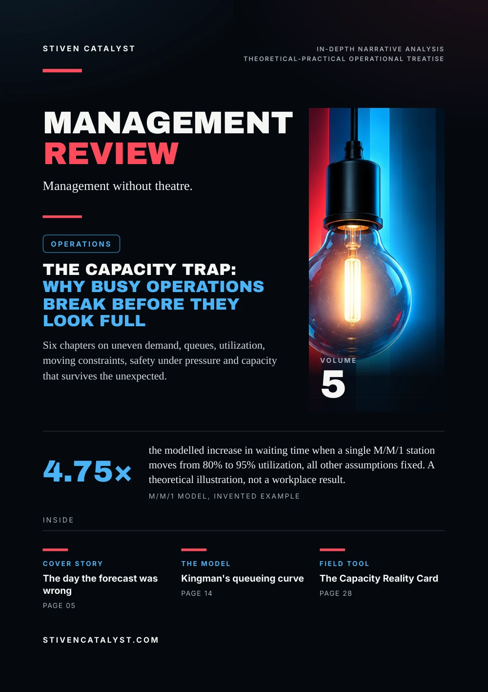
Management without theatre.
Operations
Six chapters on uneven demand, queues, utilization, moving constraints, safety under pressure and capacity that survives the unexpected.

Volume5
the modelled increase in waiting time when a single M/M/1 station moves from 80% to 95% utilization, all other assumptions fixed. A theoretical illustration, not a workplace result.M/M/1 model, invented example
stivencatalyst.com
Editorial · Volume 5
When a full schedulest ops being a plan
A busy operation can look efficient just before it becomes unable to absorb the next ordinary surprise.
How every chapter is built
- 1
The living scene
A shift, a ramp, a desk at 03:00: one piece of work followed as it actually happens, with the hand-off where it breaks. Scenes are constructed from real categories of work and say so.
- 2
The conceptual and scientific breakdown
The mechanism behind the scene, named with the model that explains it, and the research that tests it: the study, its population, its year and its limits, before it is applied anywhere else.
- 3
The operating protocol for action
What a working team can try on Monday: fields, questions, a cadence and a count, each with an owner, a next step and a return of information to the people who do the work.
The reading contract
Field
Operational contexts without invented incidents.
Evidence
Population, assumptions, boundaries and year travel with a claim.
Action
A bounded test, an owner and a verifiable customer result.
Contents
The chap ters,in three layers
Chapter IThe day the forecast was wrong05
1 SceneThe day the forecast was wrong052 BreakdownAverage demand is not arrival shape063 ProtocolPlan the window, not the average07Chapter IIThe mathematics of waiting08
1 SceneThe queue no one assigned to a team082 BreakdownLittle's Law: flow, work and time09One equation, three useful checks103 ProtocolMeasure the queue without blaming it11Chapter IIIThe price of full utilization12
1 SceneEveryone is busy. The line grows.122 BreakdownKingman: the price of variability13Four load levels, one sharp curve14The 80-vehicle warning153 ProtocolRead the curve, then test the pool16Chapter IVThe bottleneck moves17
1 SceneThe bottleneck moves172 BreakdownThe capacity of a chain is not its sum18Where the constraint changes place193 ProtocolFind the constraint that matters now20Chapter VWhen pressure attacks the standard21
1 SceneWhen speed attacks the standard212 BreakdownThe false gain of local speed22Peak pressure is time-dependent233 ProtocolPressure without silent exceptions24Chapter VIDesigning capacity for reality25
1 SceneA plan with room to move252 BreakdownBuffers are not a moral failure263 ProtocolDesign capacity for the real interval27
Also in this volume
- 04Research noteWhat capacity models are allowed to claim
- 28Field toolThe Capacity Reality Card
- 29Closing essayRoom to do the job well
- 30MethodModels, boundaries and limits
- 31SourcesSources and method
Research note
What capacit y modelsare allowed t o claim
An equation can reveal a mechanism. It cannot turn an invented example into a measurement of a real workplace.
The quantitative illustrations in this volume refer to simplified queueing systems. They are calculated from stated hypothetical assumptions, not extracted from any dispatcher dashboard, hotel PMS, customer order history or employer. Where a model assumes one server in steady state, it cannot simply be scaled to a fleet, a multi-counter reception or an end-to-end delivery network. Little's Law concerns long-run flow averages under specified regularity conditions. Kingman's approximation links waiting to variability and utilization for a single service station. Multi-server queues behave differently, a point examined by Whitt. The practical examples transfer questions to the model; they do not establish causal effects in the author's workplaces.
Theorem
A mathematical relation with defined variables and assumptions.
Approximation
A practical estimate whose accuracy depends on the model.
Hypothesis
An operational idea awaiting measurement in the real system.
A queue is not necessarily waste. Some time protects safe sequencing, required inspections and service quality. The managerial task is to distinguish necessary control from preventable delay. A demand-capacity model should show exclusions, missing data, time window, operational authority and the downstream outcome it is intended to improve.
State the unit, boundary, time window and assumptions before trusting the number.
Sources: John D. C. Little, Operations Research 9(3), 1961; J. F. C. Kingman, Mathematical Proceedings of the Cambridge Philosophical Society 57(4), 1961; Ward Whitt, Management Science 38(5), 1992; NHS England, 2026
Little (1961, 2011), Kingman (1961, 1962), Whitt (1992, 1993) and NHS England's demand and capacity models; full references on the sources page.
- 1Scene
- 2Breakdown
- 3Protocol
Chapter I · The day the forecast was wrong
The day the forecastwas wrong
The plan says enough people are rostered. The work arrives in a different shape.
Constructed scene, not a documented personal event
A dispatch shift begins with a forecast, a departure schedule and a set of loading windows. The roster looks adequate. Then several departures need attention at once, a few drivers arrive later than planned and one prepared load is not yet usable. The team has not suddenly forgotten how to work. The distribution of work across time no longer resembles the average used for planning. The person closest to the loading area sees distinct queues: work waiting for preparation, vehicles waiting for permission to proceed and exceptions waiting for a decision. A manager looking only at the total number of planned tours may see an apparently modest gap. A manager on the ramp sees that capacity cannot be teleported from a quiet period into the congested window.
The author has documented work with last-mile loading, short-notice driver availability, ramp-up and days when demand exceeded forecasts. The clock, sequence and cause in this scene are illustrative. There is no verified daily volume or outcome that could be supplied responsibly as a case study.
Capacity that exists on paper but not at the required time is not available capacity.
Documented categories of last-mile work; the particular scene is hypothetical. The essay named below tells a high-volume day from the dispatch desk.
- 1Scene
- 2Breakdown
- 3Protocol
Chapter I · The day the forecast was wrong
Average demandis not arrival shape
Two shifts can receive the same total work and need different capacity because their peaks occur at different times. A daily mean removes the information that makes a shift difficult. Imagine 100 requests divided across ten equal windows. Ten in every window and a pattern of two, two, twenty-four, twenty-four and smaller values elsewhere share the same total. The second creates a queue if processing cannot follow the surge.
Synthetic example from stated assumptions, not a measurement
Two arrival profiles with the same 100 requests, busiest window
Operations science distinguishes the arrival process, the service process and the resources that can perform that service. Effective capacity includes training, authorization, equipment availability, set-up or travel time and constraints between steps. A vehicle count is not an effective departure rate; a number of reception colleagues does not tell us how many distinct types of requests they can finish at a peak. A useful capacity review therefore uses matched intervals: compare demand and effective service ability for each operational window. Where job types compete for different skills, a single total hides bottlenecks. Record both what has arrived and what is actually ready to be worked.
A forecast can be correct for the day and still be unusable for the hour.
Sources: Wallace J. Hopp & Mark L. Spearman, Waveland Press, 2011; NHS England, 2026
Arrival, service and effective capacity after Hopp and Spearman's Factory Physics and NHS England's demand and capacity guidance; the two profiles are invented.
- 1Scene
- 2Breakdown
- 3Protocol
Chapter I · The day the forecast was wrong
Plan the window,not the average
Five checks before concluding that the scheduled resources match the work.
Define the unit
Tour ready to load, bag group, request or case; do not mix unlike workloads into one count.
Choose short intervals
Windows appropriate to the process; find the peak arrival concentration, not just the daily total.
Estimate effective capacity
Subtract known unavailability and constraints without assuming all people are interchangeable.
Inspect work at the boundary
How many jobs are truly ready, waiting, active, blocked and completed at each point?
Set a response owner
Who can coordinate a lawful capacity adjustment, and how the team will know the plan changed.
Record the forecast and the actual arrivals by interval, with source, time zone and exclusion rule. A forecast-error percentage says little about whether the missed work arrived in a critical window; do not turn a small miss into evidence of poor effort by a colleague. Safety and legally required breaks are constraints, not spare capacity.
The useful question is not “Did we have enough people today?” but “Could the required work be served when it arrived?”
Sources: NHS England, 2026; Wallace J. Hopp & Mark L. Spearman, Waveland Press, 2011
Practice proposed by the editors after NHS England's demand and capacity approach and Factory Physics; not a documented employer SOP.
- 1Scene
- 2Breakdown
- 3Protocol
Chapter II · The mathematics of waiting
The queue no oneassigned t o a team
One department has completed its task. The next person cannot begin.
Hypothetical service example, not a named hotel incident
At an imaginary service desk, a request has been logged but needs an answer from another function. The receptionist finishes registering the matter and turns to the next guest. The request sits in a queue not shown by the counter's local service-time metric. The customer still experiences waiting, even though the first employee has completed the assigned step. The same geometry occurs in wholesale and last-mile delivery: the order is accepted but not ready for preparation; the load is physically present but awaits clarification; an exception has been reported but has not received a decision. The unit moves forward only when both the work and the information needed for the next step arrive.
This constructed scene uses work categories from the author's background, not a claim that a particular hotel delayed a guest or that a specified order was lost. The purpose is to identify which queue is outside the owner's field of view. Counting only the minutes spent processing a request misses the time it occupies the entire system.
A team may complete its local task while the customer's clock keeps running.
Constructed scene, after Little (1961, 2011) and the value-stream volumes; the essay named below tells the night desk's version.
- 1Scene
- 2Breakdown
- 3Protocol
Chapter II · The mathematics of waiting
Lit tle's Law:flow, work and time
In a stable boundary with coherent long-run averages, throughput and time determine the average amount of work inside.
John D. C. Little's 1961 result expresses a conservation relation for queueing processes under mathematical conditions. It is not an instruction to accelerate a specific employee. Its main operational value is forcing managers to agree on the boundary: where a job enters, where it leaves and which waiting states are included. If a process completes on average 24 requests per hour and each request stays inside its boundary for 0.5 hour, the implied average work-in-process is 12 requests. This is a fully synthetic illustration of the relation; it says nothing about service times, delays or staffing at a particular hotel or warehouse.
The throughput rate should be consistent with the measured system during the period of analysis. During an accumulating backlog, incoming demand and completed throughput are not interchangeable. Under severe transients, a snapshot of queue length should not be plugged into the long-run formula as though the queue were stable.
The formula disciplines the definition of the process. It does not diagnose the cause of waiting.
Sources: John D. C. Little, Operations Research 9(3), 1961; John D. C. Little, Operations Research 59(3), 2011
Little, Operations Research 9(3), 383–387 (1961); Little (2011) for the conditions. The 24 × 0.5 = 12 calculation is hypothetical.
- 1Scene
- 2Breakdown
- 3Protocol
Chapter II · The mathematics of waiting
One equation,three useful checks
A reproducible illustration with explicit assumptions, not a performance claim.
Synthetic example from stated assumptions, not a measurement
Average completion rate: 24 cases/hour
Long-run throughput λ.
Average total time: 0.5 hour/case
Time in system W.
Implied average cases: 12
L = 24 × 0.5.
If time becomes 0.75 h: 18 cases
Only if throughput remains 24/h.
The first three rows describe one hypothetical stable boundary. The fourth is a scenario, not a forecast: holding throughput at 24 cases per hour while average elapsed time increases to 45 minutes implies 18 cases in the system. It does not mean 18 workers are needed; cases may be waiting rather than actively processed. A careful analyst checks conservation first. Are arrivals, departures and the opening and closing queue reconciled? Do all timestamps use the same clock? Are cancelled, abandoned, rerouted or reworked jobs treated consistently? Is the observed period long enough to describe the flow of interest?
A mathematically correct equation can still produce a misleading answer when its units and boundary are wrong.
Sources: John D. C. Little, Operations Research 9(3), 1961; John D. C. Little, Operations Research 59(3), 2011
Little (1961, 2011); all case counts and durations on this page are synthetic.
- 1Scene
- 2Breakdown
- 3Protocol
Chapter II · The mathematics of waiting
Measure the queuewithout blaming it
A compact measurement sequence that does not confuse activity, waiting and failure.
Select one service boundary
A clearly defined kind of work, followed from release into the process to usable completion.
Capture entry and exit
Permitted, consistent timestamps and a declared convention for interruptions.
Count pending work
Waiting, active, held for information and finished, at agreed intervals.
Reconcile the flow
Opening queue + new arrivals − completions − documented exits = closing queue.
Separate necessary checks
Keep legally required, safety and quality steps; examine avoidable rework and uncertainty.
Review with the owners
Ask both sender and receiver whether the numbers describe the actual handover.
Avoid collecting private identifiers in a public case study. A small, properly anonymised sample can be enough to demonstrate the method. If the queue cannot be measured reliably, write “not measured”, state the missing fields and propose a modest data-quality check.
The first output of a queue study should be a trustworthy description, not a verdict about staff effort.
Sources: John D. C. Little, Operations Research 9(3), 1961; NHS England, 2026
Editorial protocol after Little (1961) and NHS England's demand and capacity measurement guidance.
- 1Scene
- 2Breakdown
- 3Protocol
Chapter III · The price of full utilization
Everyone is busy.The line grows.
The last few points of utilization may cost more service time than managers expect.
Constructed illustration, a single workstation
Imagine one processing station that can finish twelve standard jobs per hour when continuously occupied. On a quiet day, work arrives often enough to keep the station useful, and small gaps absorb variation. As arrivals become heavier, the gaps disappear. A long task, late release or batch of simultaneous arrivals can now push other jobs into a line. The manager sees an employee working continuously and concludes that the desk is efficient. The next employee sees an overflowing queue. Both observations can be true: high utilization explains how much capacity is consumed; it does not, by itself, measure the service experienced by those waiting.
The single-station example is intentionally abstract. Last-mile operations involve many workers, vehicles, constraints and changing times. The model can illustrate the mechanism without serving as a valid numerical prediction for the author's dispatcher work.
There is a point at which using every available minute makes the next minute much less reliable.
Research framework: Kingman (1961, 1962), Whitt (1992); the workstation and demand are hypothetical. The essay named below is about a fleet no dashboard shows.
- 1Scene
- 2Breakdown
- 3Protocol
Chapter III · The price of full utilization
Kingman: the priceof variabilit y
For a single-server G/G/1 queue, a classic approximation connects mean waiting to utilization and variability.
In plain language, the model combines three influences. Greater variation in arrivals or task times raises the waiting burden. Higher utilization reduces the available buffer. Longer processing times scale the size of the delay. The formula is an approximation for a defined single-station queue and is especially useful for showing heavy-traffic sensitivity; it is not a universal capacity target. Take a hypothetical station with exponential arrivals and service times and a mean service time of five minutes. The variability multiplier is then one. The calculation on the next page is exact for that M/M/1 case in steady state; the G/G/1 expression stays an approximation, ρ/(1−ρ) is not a “productivity score”, and five minutes must not be transferred to unloading, driving or a front desk as if they were identical.
Near capacity, variability is no longer a minor inconvenience. It becomes a queue amplifier.
Sources: J. F. C. Kingman, Mathematical Proceedings of the Cambridge Philosophical Society 57(4), 1961; J. F. C. Kingman, Journal of the Royal Statistical Society, Series B 24(2), 1962; Wallace J. Hopp & Mark L. Spearman, Waveland Press, 2011
Kingman (1961, 1962); the VUT form of the approximation as in Factory Physics. Not a measured profile of any employer.
- 1Scene
- 2Breakdown
- 3Protocol
Chapter III · The price of full utilization
Four load levels,one sharp curve
Under a hypothetical steady M/M/1 queue with a mean service time of five minutes, the expected wait before service is five minutes times ρ/(1−ρ).
Synthetic example from stated assumptions, not a measurement
Expected wait before service, minutes, by utilization (M/M/1, te = 5 min)
The load factor ρ/(1−ρ) is 2.33 at 70%, 4.00 at 80%, 9.00 at 90% and 19.00 at 95%. With this one-station model, moving from 80% to 95% multiplies the predicted queue wait by 4.75, assuming the same service time and distributional assumptions. That is not a claim that warehouse loading time, route delay or a multi-employee reception will multiply by 4.75. It is a demonstration of non-linear congestion near saturation.
High utilization makes waiting sensitive to small disruptions; it does not prove that any particular staffing plan is wrong.
Source: J. F. C. Kingman, Mathematical Proceedings of the Cambridge Philosophical Society 57(4), 1961
Calculation from the classical M/M/1 special case, Wq = te × ρ/(1−ρ); Kingman (1961) gives the general single-server approximation. All scenarios are hypothetical.
- 1Scene
- 2Breakdown
- 3Protocol
Chapter III · The price of full utilization
The 80-vehiclewarning
A fleet is not one server, and a multi-worker operation should not inherit a single-station prediction.
Ward Whitt's 1992 research on the efficiency of multi-server service systems shows why the size and structure of a service system matter when choosing a utilization policy. Larger pools of servers can gain efficiency from pooling demand, and higher variability tends to reduce the utilization compatible with a given service standard. That is more nuanced than declaring that all teams must run at 80%, or that any observed utilization above 90% is automatically unacceptable. Whitt's 1993 paper developed approximations for GI/G/m queues, where multiple identical servers serve a common queue under specified assumptions. Real transport networks often have geographic separation, heterogeneous vehicles, different skills, deadlines and time-dependent demand. These constraints limit how much pooling is possible. A spare driver in one location is not necessarily spare capacity for another route.
Pooling
Shared flexible capacity may absorb variation better.
Friction
Skill, location, route and handover rules can prevent sharing.
Service
Choose capacity against waiting, quality and risk targets.
Pool resources only where the work and the rules actually allow them to be pooled.
Sources: Ward Whitt, Management Science 38(5), 1992; Ward Whitt, Production and Operations Management 2(2), 1993
Whitt, Management Science 38(5), 1992, and Production and Operations Management 2(2), 1993; the three cards are editorial.
- 1Scene
- 2Breakdown
- 3Protocol
Chapter III · The price of full utilization
Read the curve,then test the pool
Use the single-station curve to ask why congestion accelerates; use a validated multi-resource model, process measurements or a controlled test to estimate the impact on a real workforce.
Locate the station that is near its limit
Measured utilization by window, with the service time and its variation.
Separate the two levers
Less variability in arrivals or tasks, or more effective capacity; each has a different cost.
Check what can actually be pooled
Skills, locations, routes, authorisations and handover rules that prevent sharing.
Set the service target first
Waiting, quality and risk limits; the utilization that fits them follows.
Test one change, one window
A bounded pilot with an owner, before any budget or staffing commitment.
“More vehicles” is not a conclusion until the limiting activity, timing and permissions are understood. A utilization number without its service target is a description of effort, not a decision.
The curve tells you where waiting becomes fragile. Only the real system tells you what to change.
Sources: J. F. C. Kingman, Mathematical Proceedings of the Cambridge Philosophical Society 57(4), 1961; Ward Whitt, Management Science 38(5), 1992; Ward Whitt, Production and Operations Management 2(2), 1993
Editorial protocol after Kingman (1961) and Whitt (1992, 1993); the author's PDF folds these steps into its research page.
- 1Scene
- 2Breakdown
- 3Protocol
Chapter IV · The bottleneck moves
The bot tleneckmoves
Solving one constrained step can expose another one a few metres, minutes or departments away.
Hypothetical last-mile flow, no claimed performance result
At a fictional loading point, the first pressure is on preparing the load. Management adds preparation help and the work reaches the ramp sooner. The next day the preparation queue is visibly smaller, but departures have not improved. More loads now wait for checks and release. The constraint has moved, or perhaps the original measurement missed it. A manager celebrating the reduction in preparation time has a true local result. The recipient of the complete service may see no gain. This is why adding people to the activity with the most visible queue is not automatically a whole-system solution. The answer depends on which step controls the maximum rate of completed, usable work, at what time and under which quality conditions.
The author's last-mile experience involved preparation, loading, missing bags, ramp order and departures. There is no documented before-and-after staffing experiment with the specific rates in this story. The scene is deliberately invented to illustrate a coupled flow.
The line you made shorter may simply have reappeared at the next handover.
Research framework: Hopp and Spearman, Factory Physics. All events and implied outcomes are constructed; the essay named below follows a mistake across departments.
- 1Scene
- 2Breakdown
- 3Protocol
Chapter IV · The bottleneck moves
The capacit y of a chainis not its sum
An end-to-end flow is limited by the slowest required step even when other parts appear under-used: for an idealised series of steps with stable rates and no alternate path, sustained throughput cannot exceed the smallest step capacity.
Synthetic example from stated assumptions, not a measurement
A three-step flow, usable jobs per hour; the chain is capped by release
Imagine a simple three-step flow: preparation can provide 75 usable jobs per hour, verification can handle 70 and release can finish 55. Under the stated simplification, the chain cannot sustainably release more than 55 per hour. Raising preparation from 75 to 90 changes nothing about that bound: a local KPI improves while the customer waits just as long. The next question is not “Which department is least busy?” but “What stops the finished order crossing the boundary the customer cares about?”, and the answer may be information, not motion.
Improving the largest capacity rarely fixes a smaller capacity downstream.
Source: Wallace J. Hopp & Mark L. Spearman, Waveland Press, 2011
Illustrative arithmetic and flow logic after Factory Physics; hypothetical capacities, no recorded operating dataset.
- 1Scene
- 2Breakdown
- 3Protocol
Chapter IV · The bottleneck moves
Where the constraintchanges place
A simple serial-flow model to show why improvement needs a second measurement after the change. The rates are invented; the exercise is deterministic and ignores randomness, inventories, rework and job-mix differences.
Synthetic example from stated assumptions, not a measurement
A · first review: 75 / 70 / 55 → chain 55
Release restricts the whole flow.
B · faster prep: 90 / 70 / 55 → chain 55
Preparation speeds up; the total limit does not move.
C · release improved: 90 / 70 / 72 → chain 70
Improving release exposes verification as the lowest step.
D · check deteriorates: 90 / 52 / 72 → chain 52
The checking rate falls and becomes the new constraint.
In real last-mile work, a queue can migrate between preparation, waiting for a decision, loading, departure and a tour in progress. In a hotel, the limiting service may move between front desk availability, a specialist response or the next shift's capacity. A manager needs a flow-level measure to distinguish such changes from a problem that merely appears in a new dashboard.
After every local speed-up, re-measure the complete chain.
Source: Wallace J. Hopp & Mark L. Spearman, Waveland Press, 2011
Synthetic serial-line example inspired by Hopp and Spearman; values are teaching inputs, not validated estimates for field operations.
- 1Scene
- 2Breakdown
- 3Protocol
Chapter IV · The bottleneck moves
Find the constraintthat mat ters now
A repeatable sequence for deciding where to investigate, rather than chasing the longest-looking queue.
Name the customer outcome
What completed, usable work means, and the deadline.
Draw the necessary steps
Release decisions and handovers too, not only visible tasks.
Count arrivals and completions
Queues and effective capacity in the same short windows.
Check actual blockage
Waiting for skill, equipment, information, safe access or authorization?
Test a focused relief
One approved condition changed, no control reduced; note the downstream effect.
Measure the next boundary
Where work accumulates after the change, and whether the customer outcome improves.
A bottleneck label is provisional until the local conditions and time window are known. With parallel branches or reroutes, a minimum-capacity equation is not enough: observation, data checks and perhaps simulation are needed, and always a named owner for the next decision.
Manage the rate of completed, usable service. Local speed is only one possible contributor.
Sources: Wallace J. Hopp & Mark L. Spearman, Waveland Press, 2011; Ward Whitt, Production and Operations Management 2(2), 1993
Editorial protocol informed by Factory Physics and multi-server queue research; not an employer-specific procedure.
- 1Scene
- 2Breakdown
- 3Protocol
Chapter V · When pressure attacks the standard
When speedat tacks the standard
The more urgent the schedule becomes, the easier it is to confuse a completed task with correctly completed work.
Constructed scene; safety and quality requirements stay binding
A hypothetical departure window is running late. A prepared trolley is almost ready, a driver is waiting and colleagues are answering several questions at once. Someone proposes skipping a final verification to recover time. The suggestion sounds operational: reduce a task now and the vehicle can leave sooner. But if the load is incomplete, the shortcut may transfer the loss to delivery, recovery work and the customer. In the author's real last-mile context, standards covered trolley organization, reporting missing bags and the handling of work in designated zones. Demand and ramp-up created real coordination pressure. There is no verified episode in which the author accepted the proposed shortcut, nor measured causal impact of one hypothetical check on delay or incomplete orders.
Pressure does not erase the difference between optional effort and required control. Managers can adjust sequencing and capacity through authorized methods. They should not redefine a safety- or quality-critical step as waste merely because the queue is visible.
A quicker departure is not a better service if it exports an unresolved defect.
Editorial illustration of an operational trade-off, not a specific employer incident; framework Factory Physics. The essay named below is about damage worked on, not hidden.
- 1Scene
- 2Breakdown
- 3Protocol
Chapter V · When pressure attacks the standard
The false gainof local speed
A useful capacity measure counts usable output and the cost of work that comes back. Gross throughput counts all attempted completions; good throughput counts results that meet the agreed customer and quality requirements. The gap matters when defects trigger repacking, new handling, explanations, complaint work or another turn through the process.
Synthetic example from stated assumptions, not a measurement
Before change: 100 gross, 94 good, 94.0% first pass
One hypothetical window.
After speed-up: 110 gross, 97 good, 88.2% first pass
Good output rose by three; first-pass acceptance fell.
Suppose an imaginary workstation processes 100 items and only 94 are accepted without rework: first-pass acceptance is 94%. If a change raises gross output to 110 but only 97 are accepted, good output increased by three while first-pass acceptance fell to about 88.2%. These numbers are fictional and cannot be used to judge a named driver or an improvement in the author's workplace. Neither ratio proves the change is good or bad without labour input, risk, costs, service impact and demand. The example teaches a measurement boundary: if managers report only “more work done”, they can overlook the burden shifted to the next team. Quality, safety and employee fatigue are constraints on acceptable solutions, not just secondary scorecards.
Measure speed together with the amount of work the next person can use without correction.
Source: Wallace J. Hopp & Mark L. Spearman, Waveland Press, 2011
Synthetic first-pass example; interpretation after Factory Physics and the value-stream measures of Volume 2; no local causal inference.
- 1Scene
- 2Breakdown
- 3Protocol
Chapter V · When pressure attacks the standard
Peak pressureis time-dependent
Stationary averages can conceal the timing of congestion even in rigorously studied service models. Eick, Massey and Whitt (1993) studied time-dependent arrival rates in an infinite-server queue. Their paper shows that the number of busy resources at a moment can depend on the service-time distribution and the history of arrivals, not just the arrival rate visible at that instant.
This is a mathematical model of a particular system, not a direct measurement of loading ramps or hotel demand. For practical operations, the transferable question is powerful: when does work enter, how long does it remain active and at what times does the system carry its largest unfinished workload? A surge may continue to influence congestion after new arrivals have slowed, because work that entered during the peak has not yet finished. The model assumes infinitely many servers and therefore removes waiting due to a capacity limit. Real operations have finite resources, making its numerical predictions unsuitable as direct estimates of real queues. Its value here is to underscore that staffing based only on a daily mean or a peak arrival count may overlook the workload already occupying the system.
Arrival profile
Demand varies by window; daily averages erase sequence.
Service duration
Tasks overlap in time; the tail of a surge may persist.
Capacity limit
Real work has finite skills, resources and permissions.
A peak can end on the arrival chart before it ends in the work.
Source: Stephen G. Eick, William A. Massey & Ward Whitt, Operations Research 41(4), 1993
Eick, Massey and Whitt, Operations Research 41(4), 731–742 (1993); the operational application is interpretive.
- 1Scene
- 2Breakdown
- 3Protocol
Chapter V · When pressure attacks the standard
Pressure withoutsilent excep tions
Plan the response to a peak while keeping the non-negotiable conditions visible.
Name the protected standards
Required controls, legal rest rules and safety limits, before the shift.
Set a visible trigger
A measured queue, unfinished workload or service threshold, not an impression.
Separate response lanes
Safety concerns follow approved escalation; routine congestion uses authorized capacity and sequence choices.
Rebalance only usable capacity
Skills, place, timing and authorization, before moving help.
Record trade-offs
Accepted completions, backlog, rework and the customer effect, together.
Close and learn
What changed, what stayed open, whether a forecast or standard needs review.
Treat exception reporting as information. It is not proof that a colleague is careless, and it is not permission to ignore deliberate breaches of critical procedures. An honest report about a constraint should improve the plan, not make the reporter disappear from the chart.
Resilience is a method for responding to pressure, not a license to bypass the standard.
Sources: J. F. C. Kingman, Mathematical Proceedings of the Cambridge Philosophical Society 57(4), 1961; Stephen G. Eick, William A. Massey & Ward Whitt, Operations Research 41(4), 1993
Editorial peak-response protocol informed by the variability models above and everyday operational safeguards; local authorization always governs.
- 1Scene
- 2Breakdown
- 3Protocol
Chapter VI · Designing capacity for reality
A plan withroom t o move
The ideal roster is not necessarily the roster that survives an ordinary bad hour.
Hypothetical planning meeting, no verified employer result
A planning team has enough scheduled resources for the expected volume. Every assigned minute has a job. The plan looks economical. One supervisor asks a different question: what happens if arrivals cluster, a vehicle becomes unavailable or a newly trained employee needs assistance? The spreadsheet has no answer, because “available capacity” has been defined as if it were independent of the day's conditions. The team does not immediately demand more resources. First it distinguishes the work that can be shifted in time, the work that cannot, and the roles that can substitute for one another. It tests whether a small reserve, an earlier quality check or a more realistic release schedule changes the end-to-end outcome. The decision is based on a scenario with assumptions, not on an inspiring target for maximum occupancy.
The author's work across last-mile, hotel shifts and wholesale coordination motivates the question, but there is no recorded instance of this precise planning meeting or a measured outcome from a particular reserve-capacity initiative.
A good plan includes a response to uncertainty, not a pretence that uncertainty has been eliminated.
Constructed scenario after Factory Physics and NHS England's demand and capacity guidance; the essay named below is the ten minutes before a shift.
- 1Scene
- 2Breakdown
- 3Protocol
Chapter VI · Designing capacity for reality
Buffers are nota moral failure
Time, capacity and limited work-in-process are three ways of coping with uncertain arrivals and service times, each with a cost: long lead times hide defects, idle resources cost money, unfinished work lengthens the wait. No universal percentage tells every service to reserve the same capacity.
Synthetic example from stated assumptions, not a measurement
A station that receives 12 jobs an hour for two hours and finishes 10 an hour accumulates four, ignoring variation, lost jobs and an initial queue. That is not a stable queue and must not be fed into Little's steady-state averages. The next planning question is the recovery window: how fast can the backlog fall once demand drops, without sacrificing safety or creating rework? NHS England's models separate required from available capacity and update as local data change; the clinical model must be adapted, not copied.
The reserve is not an idle luxury if it is what prevents a short surge from becoming a long failure.
Sources: Wallace J. Hopp & Mark L. Spearman, Waveland Press, 2011; NHS England, 2026
Buffers after Factory Physics; required versus available capacity after NHS England. The surge calculation is hypothetical, not local evidence.
- 1Scene
- 2Breakdown
- 3Protocol
Chapter VI · Designing capacity for reality
Design capacit yfor the real interval
An operating model that tests the forecast, the queue, the service and the recovery, in that order.
Choose the service promise
Customer result and deadline, not a utilization target.
Measure arrival and service profiles
Matched short intervals, job categories, effective availability.
Identify constraints
Physical capacity, skills and locations, information gaps, required controls.
Run three bounded scenarios
Expected period, credible surge, recovery after surge; all assumptions disclosed.
Select authorized actions
Capacity, sequencing or work-release changes, with named owners.
Test and tell back
Backlog, accepted output, exceptions and customer effect compared; the decision reported to the team.
The target is not “as much usage as possible” but adequate service with transparent limits, safe execution and the ability to recover. For a fleet or a multi-team operation the single-server formula is a teaching tool only; use local data and a fitting model before committing budgets, staffing or service promises.
Capacity planning is complete only when the team knows what it will do when the forecast becomes wrong.
Sources: John D. C. Little, Operations Research 9(3), 1961; J. F. C. Kingman, Mathematical Proceedings of the Cambridge Philosophical Society 57(4), 1961; Ward Whitt, Management Science 38(5), 1992; Wallace J. Hopp & Mark L. Spearman, Waveland Press, 2011; NHS England, 2026
Original editorial procedure synthesising Little, Kingman, Whitt, Factory Physics and NHS England guidance; not field-tested.
Field tool
The Capacit yRealit y Card
One operating window, one service promise and one decision that can be checked against reality. Write “not measured” where data are absent.
01Flow and customerwhich work type, arrival boundary and promised outcome?
02Window and baselinewhat time interval? what is actual demand and what is forecast?
03Effective capacitywhich people or resources are usable in that window, under which constraints?
04Queue and qualitywhat is waiting, blocked, accepted, returned for rework or still open?
05Surge and recoverywhat if arrivals cluster? how long could the backlog take to clear?
06Decision and ownerwhat authorized change is proposed, by whom and for which checkpoint?
07Tell back and learningwho informs the frontline of the result and the next review?
Sources: John D. C. Little, Operations Research 9(3), 1961; J. F. C. Kingman, Mathematical Proceedings of the Cambridge Philosophical Society 57(4), 1961; Wallace J. Hopp & Mark L. Spearman, Waveland Press, 2011; NHS England, 2026
Use an anonymised example for publication; never copy guest, payment, driver identifiers or confidential operational exports into a public tool. A proposed field worksheet, not a validated capacity algorithm.
Closing essay
Room t o dothe job well
An operation does not become resilient because its schedule is full. It becomes resilient when its promises can survive ordinary uncertainty.
There is a familiar appeal in a perfectly occupied plan. Every vehicle assigned, every desk staffed to the predicted workload, every team visibly busy. The plan appears disciplined because nothing seems unused. Yet the number of occupied minutes is not the customer's experience. A customer waits in the gaps between our definitions of completion. An employee absorbs the surprises that an average has hidden. A supervisor encounters a line that cannot be shortened by asking people to hurry. Little gives us a language for flow and time. Kingman shows why utilization and variability compound waiting in the single-station model. Whitt warns that pooling and service scale change the calculation. Factory Physics reminds us that processes behave as systems of material, information, resources and variation. None of these sources knows the author's actual loading rates or the number of conversations a particular night-shift colleague completed. Their purpose in this volume is not to fabricate measurements but to improve the questions managers ask.
Some operating problems need more capacity. Others need work released at a better time, clearer exceptions, usable information, an appropriate skill match or a standard that new colleagues can follow without constant rescue. A queue can be a signal of genuine shortage, a broken handover or a safety-critical step doing exactly what it is supposed to do. The diagnosis must precede the solution. A full system will always be impressive to the person reading a resource-utilization report. The more difficult test is whether the team can respond to an imperfect day without sacrificing quality or transferring the failure to someone else. The capacity worth defending is not the capacity to keep everybody occupied. It is the capacity to keep the service promise.
Build enough room for reality. Then use the room to do the work correctly.
Editorial conclusion. A system does not become resilient by keeping everyone busy; it becomes resilient by knowing how much pressure it can absorb before performance begins to fail.
Method
Models, boundariesand limits
An evidence-informed editorial synthesis, not a field experiment. Every case with a clock time, queue, station, staffing level or numerical outcome is labelled synthetic or hypothetical.
Theorems and approximations
Little (1961, 2011) is an exact relation under its conditions; Kingman (1961, 1962) and Whitt (1993) are approximations for defined queues; the M/M/1 waits are exact for that special case.
Scope of the models
The 80% to 95% waiting curve applies to a specified single-server queue, not to a real fleet; Eick, Massey and Whitt (1993) assume infinitely many servers.
Guidance
Factory Physics and NHS England's demand and capacity models are used as comparative planning guidance; the clinical models must be adapted, not copied.
The author's workplaces
No confidential operational values were used, and no causal result is attributed to any employer; the scenes name documented categories of work only.
Every calculation in this volume can be checked by hand: 24 × 0.5 = 12; 5 × ρ/(1−ρ) at 70, 80, 90 and 95 per cent; the minimum of 75, 70 and 55; 94 of 100 and 97 of 110; (12 − 10) × 2. Editorial standard: a theorem, an approximation and a hypothesis are named as such, and the sentence stops claiming where the model stops applying.
Sources: John D. C. Little, Operations Research 9(3), 1961; John D. C. Little, Operations Research 59(3), 2011; J. F. C. Kingman, Mathematical Proceedings of the Cambridge Philosophical Society 57(4), 1961; J. F. C. Kingman, Journal of the Royal Statistical Society, Series B 24(2), 1962; Ward Whitt, Production and Operations Management 2(2), 1993; Stephen G. Eick, William A. Massey & Ward Whitt, Operations Research 41(4), 1993; Wallace J. Hopp & Mark L. Spearman, Waveland Press, 2011; NHS England, 2026
Every source is cited at its DOI or page on the next page; the arithmetic was re-checked for the site.
Sources and method
Where the claimscome from
The figures in this volume come from the sources below, each with its year. The scenes are constructed; the protocols are proposals; what is research is named as research.
- A Proof for the Queuing Formula: L = λWJohn D. C. Little, Operations Research 9(3), 1961https://doi.org/10.1287/opre.9.3.383
- Little's Law as Viewed on Its 50th AnniversaryJohn D. C. Little, Operations Research 59(3), 2011https://doi.org/10.1287/opre.1110.0940
- The single server queue in heavy trafficJ. F. C. Kingman, Mathematical Proceedings of the Cambridge Philosophical Society 57(4), 1961https://doi.org/10.1017/S0305004100036094
- On Queues in Heavy TrafficJ. F. C. Kingman, Journal of the Royal Statistical Society, Series B 24(2), 1962https://doi.org/10.1111/j.2517-6161.1962.tb00465.x
- Understanding the Efficiency of Multi-Server Service SystemsWard Whitt, Management Science 38(5), 1992https://doi.org/10.1287/mnsc.38.5.708
- Approximations for the GI/G/m QueueWard Whitt, Production and Operations Management 2(2), 1993https://doi.org/10.1111/j.1937-5956.1993.tb00094.x
- The Physics of the Mt/G/∞ QueueStephen G. Eick, William A. Massey & Ward Whitt, Operations Research 41(4), 1993https://doi.org/10.1287/opre.41.4.731
- Factory Physics, 3rd editionWallace J. Hopp & Mark L. Spearman, Waveland Press, 2011https://factoryphysics.com/books/factory-physics-3rd-edition/
- Demand and capacity models (service-level demand and capacity planning)NHS England, 2026https://www.england.nhs.uk/ourwork/demand-and-capacity/service-level-demand-and-capacity-planning/models/
Each figure was checked for its year, its publisher and what exactly it measures, at the full text where it could be opened. Where the publisher's page could not be opened, the figure was checked against independent summaries and is marked “via”. The editors' interpretation is marked “Our reading”. No figure of the author's own workplaces is claimed.
Management without theatre.
Every volume, one question about operations, followed from the floor to the protocol and tested against research.
All volumes
stivencatalyst.com/magazine/operational-treatise.html
Operational Treatise · Volume 5 · October 2026 · Stiven Catalyst
 Next volume
The KPI trap: when the numbers improve but the work gets worse
Click or swipe a page to turn it. The arrow keys work too.
Operational Treatise · Volume 5
The figures of the volume
The charts of the printed pages, with their sources. Invented examples are marked as such.
Source: Invented example by the editors, so the arithmetic can be checked; not a measurement
Source: Invented example by the editors, so the arithmetic can be checked; not a measurement
Source: Invented example by the editors, so the arithmetic can be checked; not a measurement
The whole text Read the volume as text For reading on a small screen, searching or a screen reader. The same words, without the page design.
Editorial
When a full schedule st ops being a plan
A busy operation can look efficient just before it becomes unable to absorb the next ordinary surprise.
Managers often count people, vehicles, desks and available hours, compare a forecast with that capacity and call the difference a plan. The figures matter. Yet a system does not receive work in perfectly measured portions. Arrivals cluster. Tasks take unequal amounts of time. One late handover changes the start of the next activity. A resource that exists on a roster may not be available to the particular work waiting at a particular moment. This fifth volume studies how queues form, why utilization near the limit can magnify waiting and why the location of the main constraint shifts. The settings are familiar from the author's work: last-mile dispatch and loading, training during ramp-up, service handovers in hotels and coordination across wholesale activities. No workload, queue length, staffing figure or personal intervention is presented as a measured result of those employers. We use queueing theory to make one point precise and then challenge its limits: Little on flow and time, Kingman on variability and utilization at a single server, Whitt on the reality of many servers, and healthcare guidance on planning demand and capacity as an ongoing model. The last chapter puts the mathematics inside a cautious decision protocol.
Stiven Janaqi, Editor
How every chap ter is built
- The living scene. A shift, a ramp, a desk at 03:00: one piece of work followed as it actually happens, with the hand-off where it breaks. Scenes are constructed from real categories of work and say so.
- The conce
p tual and scientific breakdown. The mechanism behind the scene, named with the model that explains it, and the research that tests it: the study, its population, its year and its limits, before it is applied anywhere else. - The operating pro
t ocol for action. What a working team can try on Monday: fields, questions, a cadence and a count, each with an owner, a next step and a return of information to the people who do the work.
The reading contract
- Field. Operational contexts without invented incidents.
- Evidence. Population, assumptions, boundaries and year travel with a claim.
- Action. A bounded test, an owner and a verifiable customer result.
Research note
What capacit y models are allowed t o claim
An equation can reveal a mechanism. It cannot turn an invented example into a measurement of a real workplace.
The quantitative illustrations in this volume refer to simplified queueing systems. They are calculated from stated hypothetical assumptions, not extracted from any dispatcher dashboard, hotel PMS, customer order history or employer. Where a model assumes one server in steady state, it cannot simply be scaled to a fleet, a multi-counter reception or an end-to-end delivery network. Little's Law concerns long-run flow averages under specified regularity conditions. Kingman's approximation links waiting to variability and utilization for a single service station. Multi-server queues behave differently, a point examined by Whitt. The practical examples transfer questions to the model; they do not establish causal effects in the author's workplaces.
- Theorem. A mathematical relation with defined variables and assumptions.
- Approximation. A practical estimate whose accuracy depends on the model.
- Hypothesis. An operational idea awaiting measurement in the real system.
A queue is not necessarily waste. Some time protects safe sequencing, required inspections and service quality. The managerial task is to distinguish necessary control from preventable delay. A demand-capacity model should show exclusions, missing data, time window, operational authority and the downstream outcome it is intended to improve.
Our reading
State the unit, boundary, time window and assumptions before trusting the number.
Little (1961, 2011), Kingman (1961, 1962), Whitt (1992, 1993) and NHS England's demand and capacity models; full references on the sources page.
Sources: John D. C. Little, Operations Research 9(3), 1961; J. F. C. Kingman, Mathematical Proceedings of the Cambridge Philosophical Society 57(4), 1961; Ward Whitt, Management Science 38(5), 1992; NHS England, 2026
Chap ter I: The day the forecast was wrong
Layer 1 · The living scene
The day the forecast was wrong
The plan says enough people are rostered. The work arrives in a different shape.
Constructed scene, not a documented personal event
A dispatch shift begins with a forecast, a departure schedule and a set of loading windows. The roster looks adequate. Then several departures need attention at once, a few drivers arrive later than planned and one prepared load is not yet usable. The team has not suddenly forgotten how to work. The distribution of work across time no longer resembles the average used for planning. The person closest to the loading area sees distinct queues: work waiting for preparation, vehicles waiting for permission to proceed and exceptions waiting for a decision. A manager looking only at the total number of planned tours may see an apparently modest gap. A manager on the ramp sees that capacity cannot be teleported from a quiet period into the congested window.
The author has documented work with last-mile loading, short-notice driver availability, ramp-up and days when demand exceeded forecasts. The clock, sequence and cause in this scene are illustrative. There is no verified daily volume or outcome that could be supplied responsibly as a case study.
Our reading
Capacity that exists on paper but not at the required time is not available capacity.
Documented categories of last-mile work; the particular scene is hypothetical. The essay named below tells a high-volume day from the dispatch desk.
More in the essay: High-volume days: the standard under pressure
Layer 2 · The conceptual and scientific breakdown
Average demand is not arrival shape
Two shifts can receive the same total work and need different capacity because their peaks occur at different times. A daily mean removes the information that makes a shift difficult. Imagine 100 requests divided across ten equal windows. Ten in every window and a pattern of two, two, twenty-four, twenty-four and smaller values elsewhere share the same total. The second creates a queue if processing cannot follow the surge.
Synthetic example from stated assumptions, not a measurement
Two arrival profiles with the same 100 requests, busiest window: Evenly spread 10 / window, Peak window 24 / window.
Operations science distinguishes the arrival process, the service process and the resources that can perform that service. Effective capacity includes training, authorization, equipment availability, set-up or travel time and constraints between steps. A vehicle count is not an effective departure rate; a number of reception colleagues does not tell us how many distinct types of requests they can finish at a peak. A useful capacity review therefore uses matched intervals: compare demand and effective service ability for each operational window. Where job types compete for different skills, a single total hides bottlenecks. Record both what has arrived and what is actually ready to be worked.
Our reading
A forecast can be correct for the day and still be unusable for the hour.
Arrival, service and effective capacity after Hopp and Spearman's Factory Physics and NHS England's demand and capacity guidance; the two profiles are invented.
Sources: Wallace J. Hopp & Mark L. Spearman, Waveland Press, 2011; NHS England, 2026
Layer 3 · The operating protocol for action
Plan the window, not the average
Five checks before concluding that the scheduled resources match the work.
- Define the unit. Tour ready to load, bag group, request or case; do not mix unlike workloads into one count.
- Choose sho
r t intervals. Windows appropriate to the process; find the peak arrival concentration, not just the daily total. - Estimate effective capaci
t y. Subtract known unavailability and constraints without assuming all people are interchangeable. - Inspect work at the boundary. How many jobs are truly ready, waiting, active, blocked and completed at each point?
- S
e t a response owner. Who can coordinate a lawful capacity adjustment, and how the team will know the plan changed.
Record the forecast and the actual arrivals by interval, with source, time zone and exclusion rule. A forecast-error percentage says little about whether the missed work arrived in a critical window; do not turn a small miss into evidence of poor effort by a colleague. Safety and legally required breaks are constraints, not spare capacity.
Our reading
The useful question is not “Did we have enough people today?” but “Could the required work be served when it arrived?”
Practice proposed by the editors after NHS England's demand and capacity approach and Factory Physics; not a documented employer SOP.
Sources: NHS England, 2026; Wallace J. Hopp & Mark L. Spearman, Waveland Press, 2011
Chap ter II: The mathematics of waiting
Layer 1 · The living scene
The queue no one assigned t o a team
One department has completed its task. The next person cannot begin.
Hypothetical service example, not a named hotel incident
At an imaginary service desk, a request has been logged but needs an answer from another function. The receptionist finishes registering the matter and turns to the next guest. The request sits in a queue not shown by the counter's local service-time metric. The customer still experiences waiting, even though the first employee has completed the assigned step. The same geometry occurs in wholesale and last-mile delivery: the order is accepted but not ready for preparation; the load is physically present but awaits clarification; an exception has been reported but has not received a decision. The unit moves forward only when both the work and the information needed for the next step arrive.
This constructed scene uses work categories from the author's background, not a claim that a particular hotel delayed a guest or that a specified order was lost. The purpose is to identify which queue is outside the owner's field of view. Counting only the minutes spent processing a request misses the time it occupies the entire system.
Our reading
A team may complete its local task while the customer's clock keeps running.
Constructed scene, after Little (1961, 2011) and the value-stream volumes; the essay named below tells the night desk's version.
More in the essay: The angry guest at 2 a.m.
Layer 2 · The conceptual and scientific breakdown
Lit tle's Law: flow, work and time
In a stable boundary with coherent long-run averages, throughput and time determine the average amount of work inside.
L = λ × W L = average number of jobs inside the defined system; λ = average completed jobs per time unit; W = average total time inside
John D. C. Little's 1961 result expresses a conservation relation for queueing processes under mathematical conditions. It is not an instruction to accelerate a specific employee. Its main operational value is forcing managers to agree on the boundary: where a job enters, where it leaves and which waiting states are included. If a process completes on average 24 requests per hour and each request stays inside its boundary for 0.5 hour, the implied average work-in-process is 12 requests. This is a fully synthetic illustration of the relation; it says nothing about service times, delays or staffing at a particular hotel or warehouse.
The throughput rate should be consistent with the measured system during the period of analysis. During an accumulating backlog, incoming demand and completed throughput are not interchangeable. Under severe transients, a snapshot of queue length should not be plugged into the long-run formula as though the queue were stable.
Our reading
The formula disciplines the definition of the process. It does not diagnose the cause of waiting.
Little, Operations Research 9(3), 383–387 (1961); Little (2011) for the conditions. The 24 × 0.5 = 12 calculation is hypothetical.
Sources: John D. C. Little, Operations Research 9(3), 1961; John D. C. Little, Operations Research 59(3), 2011
Layer 2 · The conceptual and scientific breakdown
One equation, three useful checks
A reproducible illustration with explicit assumptions, not a performance claim.
Synthetic example from stated assumptions, not a measurement
- Average compl
e tion rate: 24 cases/hour. Long-run throughput λ. - Average
t otal time: 0.5 hour/case. Time in system W. - Implied average cases: 12. L = 24 × 0.5.
- If time becomes 0.75 h: 18 cases. Only if throughput remains 24/h.
The first three rows describe one hypothetical stable boundary. The fourth is a scenario, not a forecast: holding throughput at 24 cases per hour while average elapsed time increases to 45 minutes implies 18 cases in the system. It does not mean 18 workers are needed; cases may be waiting rather than actively processed. A careful analyst checks conservation first. Are arrivals, departures and the opening and closing queue reconciled? Do all timestamps use the same clock? Are cancelled, abandoned, rerouted or reworked jobs treated consistently? Is the observed period long enough to describe the flow of interest?
Our reading
A mathematically correct equation can still produce a misleading answer when its units and boundary are wrong.
Little (1961, 2011); all case counts and durations on this page are synthetic.
Sources: John D. C. Little, Operations Research 9(3), 1961; John D. C. Little, Operations Research 59(3), 2011
Layer 3 · The operating protocol for action
Measure the queue without blaming it
A compact measurement sequence that does not confuse activity, waiting and failure.
- Select one service boundary. A clearly defined kind of work, followed from release into the process to usable completion.
- Ca
p ture entry and exit. Permitted, consistent timestamps and a declared convention for interruptions. - Count pending work. Waiting, active, held for information and finished, at agreed intervals.
- Reconcile the flow. Opening queue + new arrivals − completions − documented exits = closing queue.
- Separate necessary checks. Keep legally required, safety and quality steps; examine avoidable rework and uncertainty.
- Review with the owners. Ask both sender and receiver whether the numbers describe the actual handover.
Avoid collecting private identifiers in a public case study. A small, properly anonymised sample can be enough to demonstrate the method. If the queue cannot be measured reliably, write “not measured”, state the missing fields and propose a modest data-quality check.
Our reading
The first output of a queue study should be a trustworthy description, not a verdict about staff effort.
Editorial protocol after Little (1961) and NHS England's demand and capacity measurement guidance.
Sources: John D. C. Little, Operations Research 9(3), 1961; NHS England, 2026
Chap ter III: The price of full utilization
Layer 1 · The living scene
Everyone is busy. The line grows.
The last few points of utilization may cost more service time than managers expect.
Constructed illustration, a single workstation
Imagine one processing station that can finish twelve standard jobs per hour when continuously occupied. On a quiet day, work arrives often enough to keep the station useful, and small gaps absorb variation. As arrivals become heavier, the gaps disappear. A long task, late release or batch of simultaneous arrivals can now push other jobs into a line. The manager sees an employee working continuously and concludes that the desk is efficient. The next employee sees an overflowing queue. Both observations can be true: high utilization explains how much capacity is consumed; it does not, by itself, measure the service experienced by those waiting.
The single-station example is intentionally abstract. Last-mile operations involve many workers, vehicles, constraints and changing times. The model can illustrate the mechanism without serving as a valid numerical prediction for the author's dispatcher work.
Our reading
There is a point at which using every available minute makes the next minute much less reliable.
Research framework: Kingman (1961, 1962), Whitt (1992); the workstation and demand are hypothetical. The essay named below is about a fleet no dashboard shows.
More in the essay: Leading 80+ vehicles you cannot see
Layer 2 · The conceptual and scientific breakdown
Kingman: the price of variabilit y
For a single-server G/G/1 queue, a classic approximation connects mean waiting to utilization and variability.
Wq ≈ V × U × te V = (ca² + cs²) / 2, the variability of arrivals and service; U = ρ / (1 − ρ), the utilization below 1; te = mean service time; Wq = expected queue wait
In plain language, the model combines three influences. Greater variation in arrivals or task times raises the waiting burden. Higher utilization reduces the available buffer. Longer processing times scale the size of the delay. The formula is an approximation for a defined single-station queue and is especially useful for showing heavy-traffic sensitivity; it is not a universal capacity target. Take a hypothetical station with exponential arrivals and service times and a mean service time of five minutes. The variability multiplier is then one. The calculation on the next page is exact for that M/M/1 case in steady state; the G/G/1 expression stays an approximation, ρ/(1−ρ) is not a “productivity score”, and five minutes must not be transferred to unloading, driving or a front desk as if they were identical.
Our reading
Near capacity, variability is no longer a minor inconvenience. It becomes a queue amplifier.
Kingman (1961, 1962); the VUT form of the approximation as in Factory Physics. Not a measured profile of any employer.
Sources: J. F. C. Kingman, Mathematical Proceedings of the Cambridge Philosophical Society 57(4), 1961; J. F. C. Kingman, Journal of the Royal Statistical Society, Series B 24(2), 1962; Wallace J. Hopp & Mark L. Spearman, Waveland Press, 2011
Layer 2 · The conceptual and scientific breakdown
Four load levels, one sharp curve
Under a hypothetical steady M/M/1 queue with a mean service time of five minutes, the expected wait before service is five minutes times ρ/(1−ρ).
Synthetic example from stated assumptions, not a measurement
Expected wait before service, minutes, by utilization (M/M/1, te = 5 min): 70% used 11.7, 80% used 20.0, 90% used 45.0, 95% used 95.0.
The load factor ρ/(1−ρ) is 2.33 at 70%, 4.00 at 80%, 9.00 at 90% and 19.00 at 95%. With this one-station model, moving from 80% to 95% multiplies the predicted queue wait by 4.75, assuming the same service time and distributional assumptions. That is not a claim that warehouse loading time, route delay or a multi-employee reception will multiply by 4.75. It is a demonstration of non-linear congestion near saturation.
Our reading
High utilization makes waiting sensitive to small disruptions; it does not prove that any particular staffing plan is wrong.
Calculation from the classical M/M/1 special case, Wq = te × ρ/(1−ρ); Kingman (1961) gives the general single-server approximation. All scenarios are hypothetical.
Source: J. F. C. Kingman, Mathematical Proceedings of the Cambridge Philosophical Society 57(4), 1961
Layer 2 · The conceptual and scientific breakdown
The 80-vehicle warning
A fleet is not one server, and a multi-worker operation should not inherit a single-station prediction.
Ward Whitt's 1992 research on the efficiency of multi-server service systems shows why the size and structure of a service system matter when choosing a utilization policy. Larger pools of servers can gain efficiency from pooling demand, and higher variability tends to reduce the utilization compatible with a given service standard. That is more nuanced than declaring that all teams must run at 80%, or that any observed utilization above 90% is automatically unacceptable. Whitt's 1993 paper developed approximations for GI/G/m queues, where multiple identical servers serve a common queue under specified assumptions. Real transport networks often have geographic separation, heterogeneous vehicles, different skills, deadlines and time-dependent demand. These constraints limit how much pooling is possible. A spare driver in one location is not necessarily spare capacity for another route.
- Pooling. Shared flexible capacity may absorb variation better.
- Friction. Skill, location, route and handover rules can prevent sharing.
- Service. Choose capacity against waiting, quality and risk targets.
Our reading
Pool resources only where the work and the rules actually allow them to be pooled.
Whitt, Management Science 38(5), 1992, and Production and Operations Management 2(2), 1993; the three cards are editorial.
Sources: Ward Whitt, Management Science 38(5), 1992; Ward Whitt, Production and Operations Management 2(2), 1993
Layer 3 · The operating protocol for action
Read the curve, then test the pool
Use the single-station curve to ask why congestion accelerates; use a validated multi-resource model, process measurements or a controlled test to estimate the impact on a real workforce.
- Locate the station that is near its limit. Measured utilization by window, with the service time and its variation.
- Separate the two levers. Less variability in arrivals or tasks, or more effective capacity; each has a different cost.
- Check what can actually be pooled. Skills, locations, routes, authorisations and handover rules that prevent sharing.
- S
e t the service targe t first. Waiting, quality and risk limits; the utilization that fits them follows. - Test one change, one window. A bounded pilot with an owner, before any budget or staffing commitment.
“More vehicles” is not a conclusion until the limiting activity, timing and permissions are understood. A utilization number without its service target is a description of effort, not a decision.
Our reading
The curve tells you where waiting becomes fragile. Only the real system tells you what to change.
Editorial protocol after Kingman (1961) and Whitt (1992, 1993); the author's PDF folds these steps into its research page.
Sources: J. F. C. Kingman, Mathematical Proceedings of the Cambridge Philosophical Society 57(4), 1961; Ward Whitt, Management Science 38(5), 1992; Ward Whitt, Production and Operations Management 2(2), 1993
Chap ter IV: The bot tleneck moves
Layer 1 · The living scene
The bot tleneck moves
Solving one constrained step can expose another one a few metres, minutes or departments away.
Hypothetical last-mile flow, no claimed performance result
At a fictional loading point, the first pressure is on preparing the load. Management adds preparation help and the work reaches the ramp sooner. The next day the preparation queue is visibly smaller, but departures have not improved. More loads now wait for checks and release. The constraint has moved, or perhaps the original measurement missed it. A manager celebrating the reduction in preparation time has a true local result. The recipient of the complete service may see no gain. This is why adding people to the activity with the most visible queue is not automatically a whole-system solution. The answer depends on which step controls the maximum rate of completed, usable work, at what time and under which quality conditions.
The author's last-mile experience involved preparation, loading, missing bags, ramp order and departures. There is no documented before-and-after staffing experiment with the specific rates in this story. The scene is deliberately invented to illustrate a coupled flow.
Our reading
The line you made shorter may simply have reappeared at the next handover.
Research framework: Hopp and Spearman, Factory Physics. All events and implied outcomes are constructed; the essay named below follows a mistake across departments.
More in the essay: Mistakes get lost between departments
Layer 2 · The conceptual and scientific breakdown
The capacit y of a chain is not its sum
An end-to-end flow is limited by the slowest required step even when other parts appear under-used: for an idealised series of steps with stable rates and no alternate path, sustained throughput cannot exceed the smallest step capacity.
Synthetic example from stated assumptions, not a measurement
A three-step flow, usable jobs per hour; the chain is capped by release: Preparation 75, Verification 70, Release 55, Preparation upgraded 90.
Imagine a simple three-step flow: preparation can provide 75 usable jobs per hour, verification can handle 70 and release can finish 55. Under the stated simplification, the chain cannot sustainably release more than 55 per hour. Raising preparation from 75 to 90 changes nothing about that bound: a local KPI improves while the customer waits just as long. The next question is not “Which department is least busy?” but “What stops the finished order crossing the boundary the customer cares about?”, and the answer may be information, not motion.
Our reading
Improving the largest capacity rarely fixes a smaller capacity downstream.
Illustrative arithmetic and flow logic after Factory Physics; hypothetical capacities, no recorded operating dataset.
Source: Wallace J. Hopp & Mark L. Spearman, Waveland Press, 2011
Layer 2 · The conceptual and scientific breakdown
Where the constraint changes place
A simple serial-flow model to show why improvement needs a second measurement after the change. The rates are invented; the exercise is deterministic and ignores randomness, inventories, rework and job-mix differences.
Synthetic example from stated assumptions, not a measurement
- A · first review: 75 / 70 / 55 → chain 55. Release restricts the whole flow.
- B · faster prep: 90 / 70 / 55 → chain 55. Preparation speeds up; the total limit does not move.
- C · release improved: 90 / 70 / 72 → chain 70. Improving release exposes verification as the lowest step.
- D · check d
e teriorates: 90 / 52 / 72 → chain 52. The checking rate falls and becomes the new constraint.
In real last-mile work, a queue can migrate between preparation, waiting for a decision, loading, departure and a tour in progress. In a hotel, the limiting service may move between front desk availability, a specialist response or the next shift's capacity. A manager needs a flow-level measure to distinguish such changes from a problem that merely appears in a new dashboard.
Our reading
After every local speed-up, re-measure the complete chain.
Synthetic serial-line example inspired by Hopp and Spearman; values are teaching inputs, not validated estimates for field operations.
Source: Wallace J. Hopp & Mark L. Spearman, Waveland Press, 2011
Layer 3 · The operating protocol for action
Find the constraint that mat ters now
A repeatable sequence for deciding where to investigate, rather than chasing the longest-looking queue.
- Name the cus
t omer out come. What completed, usable work means, and the deadline. - Draw the necessary steps. Release decisions and handovers too, not only visible tasks.
- Count arrivals and compl
e tions. Queues and effective capacity in the same short windows. - Check actual blockage. Waiting for skill, equipment, information, safe access or authorization?
- Test a focused relief. One approved condition changed, no control reduced; note the downstream effect.
- Measure the next boundary. Where work accumulates after the change, and whether the customer outcome improves.
A bottleneck label is provisional until the local conditions and time window are known. With parallel branches or reroutes, a minimum-capacity equation is not enough: observation, data checks and perhaps simulation are needed, and always a named owner for the next decision.
Our reading
Manage the rate of completed, usable service. Local speed is only one possible contributor.
Editorial protocol informed by Factory Physics and multi-server queue research; not an employer-specific procedure.
Sources: Wallace J. Hopp & Mark L. Spearman, Waveland Press, 2011; Ward Whitt, Production and Operations Management 2(2), 1993
Chap ter V: When pressure at tacks the standard
Layer 1 · The living scene
When speed at tacks the standard
The more urgent the schedule becomes, the easier it is to confuse a completed task with correctly completed work.
Constructed scene; safety and quality requirements stay binding
A hypothetical departure window is running late. A prepared trolley is almost ready, a driver is waiting and colleagues are answering several questions at once. Someone proposes skipping a final verification to recover time. The suggestion sounds operational: reduce a task now and the vehicle can leave sooner. But if the load is incomplete, the shortcut may transfer the loss to delivery, recovery work and the customer. In the author's real last-mile context, standards covered trolley organization, reporting missing bags and the handling of work in designated zones. Demand and ramp-up created real coordination pressure. There is no verified episode in which the author accepted the proposed shortcut, nor measured causal impact of one hypothetical check on delay or incomplete orders.
Pressure does not erase the difference between optional effort and required control. Managers can adjust sequencing and capacity through authorized methods. They should not redefine a safety- or quality-critical step as waste merely because the queue is visible.
Our reading
A quicker departure is not a better service if it exports an unresolved defect.
Editorial illustration of an operational trade-off, not a specific employer incident; framework Factory Physics. The essay named below is about damage worked on, not hidden.
More in the essay: How we worked with damage
Layer 2 · The conceptual and scientific breakdown
The false gain of local speed
A useful capacity measure counts usable output and the cost of work that comes back. Gross throughput counts all attempted completions; good throughput counts results that meet the agreed customer and quality requirements. The gap matters when defects trigger repacking, new handling, explanations, complaint work or another turn through the process.
Synthetic example from stated assumptions, not a measurement
- Before change: 100 gross, 94 good, 94.0% first pass. One hypothetical window.
- A
f ter speed-up: 110 gross, 97 good, 88.2% first pass. Good output rose by three; first-pass acceptance fell.
Suppose an imaginary workstation processes 100 items and only 94 are accepted without rework: first-pass acceptance is 94%. If a change raises gross output to 110 but only 97 are accepted, good output increased by three while first-pass acceptance fell to about 88.2%. These numbers are fictional and cannot be used to judge a named driver or an improvement in the author's workplace. Neither ratio proves the change is good or bad without labour input, risk, costs, service impact and demand. The example teaches a measurement boundary: if managers report only “more work done”, they can overlook the burden shifted to the next team. Quality, safety and employee fatigue are constraints on acceptable solutions, not just secondary scorecards.
Our reading
Measure speed together with the amount of work the next person can use without correction.
Synthetic first-pass example; interpretation after Factory Physics and the value-stream measures of Volume 2; no local causal inference.
Source: Wallace J. Hopp & Mark L. Spearman, Waveland Press, 2011
Layer 2 · The conceptual and scientific breakdown
Peak pressure is time-dependent
Stationary averages can conceal the timing of congestion even in rigorously studied service models. Eick, Massey and Whitt (1993) studied time-dependent arrival rates in an infinite-server queue. Their paper shows that the number of busy resources at a moment can depend on the service-time distribution and the history of arrivals, not just the arrival rate visible at that instant.
This is a mathematical model of a particular system, not a direct measurement of loading ramps or hotel demand. For practical operations, the transferable question is powerful: when does work enter, how long does it remain active and at what times does the system carry its largest unfinished workload? A surge may continue to influence congestion after new arrivals have slowed, because work that entered during the peak has not yet finished. The model assumes infinitely many servers and therefore removes waiting due to a capacity limit. Real operations have finite resources, making its numerical predictions unsuitable as direct estimates of real queues. Its value here is to underscore that staffing based only on a daily mean or a peak arrival count may overlook the workload already occupying the system.
- Arrival profile. Demand varies by window; daily averages erase sequence.
- Service duration. Tasks overlap in time; the tail of a surge may persist.
- Capaci
t y limit. Real work has finite skills, resources and permissions.
Our reading
A peak can end on the arrival chart before it ends in the work.
Eick, Massey and Whitt, Operations Research 41(4), 731–742 (1993); the operational application is interpretive.
Source: Stephen G. Eick, William A. Massey & Ward Whitt, Operations Research 41(4), 1993
Layer 3 · The operating protocol for action
Pressure without silent excep tions
Plan the response to a peak while keeping the non-negotiable conditions visible.
- Name the protected standards. Required controls, legal rest rules and safety limits, before the shift.
- S
e t a visible trigger. A measured queue, unfinished workload or service threshold, not an impression. - Separate response lanes. Safety concerns follow approved escalation; routine congestion uses authorized capacity and sequence choices.
- Rebalance only usable capaci
t y. Skills, place, timing and authorization, before moving help. - Record trade-offs. Accepted completions, backlog, rework and the customer effect, together.
- Close and learn. What changed, what stayed open, whether a forecast or standard needs review.
Treat exception reporting as information. It is not proof that a colleague is careless, and it is not permission to ignore deliberate breaches of critical procedures. An honest report about a constraint should improve the plan, not make the reporter disappear from the chart.
Our reading
Resilience is a method for responding to pressure, not a license to bypass the standard.
Editorial peak-response protocol informed by the variability models above and everyday operational safeguards; local authorization always governs.
Sources: J. F. C. Kingman, Mathematical Proceedings of the Cambridge Philosophical Society 57(4), 1961; Stephen G. Eick, William A. Massey & Ward Whitt, Operations Research 41(4), 1993
Chap ter VI: Designing capacit y for realit y
Layer 1 · The living scene
A plan with room t o move
The ideal roster is not necessarily the roster that survives an ordinary bad hour.
Hypothetical planning meeting, no verified employer result
A planning team has enough scheduled resources for the expected volume. Every assigned minute has a job. The plan looks economical. One supervisor asks a different question: what happens if arrivals cluster, a vehicle becomes unavailable or a newly trained employee needs assistance? The spreadsheet has no answer, because “available capacity” has been defined as if it were independent of the day's conditions. The team does not immediately demand more resources. First it distinguishes the work that can be shifted in time, the work that cannot, and the roles that can substitute for one another. It tests whether a small reserve, an earlier quality check or a more realistic release schedule changes the end-to-end outcome. The decision is based on a scenario with assumptions, not on an inspiring target for maximum occupancy.
The author's work across last-mile, hotel shifts and wholesale coordination motivates the question, but there is no recorded instance of this precise planning meeting or a measured outcome from a particular reserve-capacity initiative.
Our reading
A good plan includes a response to uncertainty, not a pretence that uncertainty has been eliminated.
Constructed scenario after Factory Physics and NHS England's demand and capacity guidance; the essay named below is the ten minutes before a shift.
More in the essay: Ten minutes before the shift: what the team needs to know before the work starts
Layer 2 · The conceptual and scientific breakdown
Buffers are not a moral failure
Time, capacity and limited work-in-process are three ways of coping with uncertain arrivals and service times, each with a cost: long lead times hide defects, idle resources cost money, unfinished work lengthens the wait. No universal percentage tells every service to reserve the same capacity.
Synthetic example from stated assumptions, not a measurement
4 jobs backlog after a synthetic surge: (arrivals − completions) × time = (12/h − 10/h) × 2 h
A station that receives 12 jobs an hour for two hours and finishes 10 an hour accumulates four, ignoring variation, lost jobs and an initial queue. That is not a stable queue and must not be fed into Little's steady-state averages. The next planning question is the recovery window: how fast can the backlog fall once demand drops, without sacrificing safety or creating rework? NHS England's models separate required from available capacity and update as local data change; the clinical model must be adapted, not copied.
Our reading
The reserve is not an idle luxury if it is what prevents a short surge from becoming a long failure.
Buffers after Factory Physics; required versus available capacity after NHS England. The surge calculation is hypothetical, not local evidence.
Sources: Wallace J. Hopp & Mark L. Spearman, Waveland Press, 2011; NHS England, 2026
Layer 3 · The operating protocol for action
Design capacit y for the real interval
An operating model that tests the forecast, the queue, the service and the recovery, in that order.
- Choose the service promise. Customer result and deadline, not a utilization target.
- Measure arrival and service profiles. Matched short intervals, job categories, effective availability.
- Identi
f y constraints. Physical capacity, skills and locations, information gaps, required controls. - Run three bounded scenarios. Expected period, credible surge, recovery after surge; all assumptions disclosed.
- Select authorized actions. Capacity, sequencing or work-release changes, with named owners.
- Test and tell back. Backlog, accepted output, exceptions and customer effect compared; the decision reported to the team.
The target is not “as much usage as possible” but adequate service with transparent limits, safe execution and the ability to recover. For a fleet or a multi-team operation the single-server formula is a teaching tool only; use local data and a fitting model before committing budgets, staffing or service promises.
Our reading
Capacity planning is complete only when the team knows what it will do when the forecast becomes wrong.
Original editorial procedure synthesising Little, Kingman, Whitt, Factory Physics and NHS England guidance; not field-tested.
Sources: John D. C. Little, Operations Research 9(3), 1961; J. F. C. Kingman, Mathematical Proceedings of the Cambridge Philosophical Society 57(4), 1961; Ward Whitt, Management Science 38(5), 1992; Wallace J. Hopp & Mark L. Spearman, Waveland Press, 2011; NHS England, 2026
Field tool
The Capacit y Realit y Card
One operating window, one service promise and one decision that can be checked against reality. Write “not measured” where data are absent.
- Flow and cus
t omer which work type, arrival boundary and promised outcome? - Window and baseline what time interval? what is actual demand and what is forecast?
- Effective capaci
t y which people or resources are usable in that window, under which constraints? - Queue and quali
t y what is waiting, blocked, accepted, returned for rework or still open? - Surge and recovery what if arrivals cluster? how long could the backlog take to clear?
- Decision and owner what authorized change is proposed, by whom and for which checkpoint?
- Tell back and learning who informs the frontline of the result and the next review?
Use an anonymised example for publication; never copy guest, payment, driver identifiers or confidential operational exports into a public tool. A proposed field worksheet, not a validated capacity algorithm.
Sources: John D. C. Little, Operations Research 9(3), 1961; J. F. C. Kingman, Mathematical Proceedings of the Cambridge Philosophical Society 57(4), 1961; Wallace J. Hopp & Mark L. Spearman, Waveland Press, 2011; NHS England, 2026
Open the tool: Last-Mile CX Control Tower
Closing essay
Room t o do the job well
An operation does not become resilient because its schedule is full. It becomes resilient when its promises can survive ordinary uncertainty.
There is a familiar appeal in a perfectly occupied plan. Every vehicle assigned, every desk staffed to the predicted workload, every team visibly busy. The plan appears disciplined because nothing seems unused. Yet the number of occupied minutes is not the customer's experience. A customer waits in the gaps between our definitions of completion. An employee absorbs the surprises that an average has hidden. A supervisor encounters a line that cannot be shortened by asking people to hurry. Little gives us a language for flow and time. Kingman shows why utilization and variability compound waiting in the single-station model. Whitt warns that pooling and service scale change the calculation. Factory Physics reminds us that processes behave as systems of material, information, resources and variation. None of these sources knows the author's actual loading rates or the number of conversations a particular night-shift colleague completed. Their purpose in this volume is not to fabricate measurements but to improve the questions managers ask.
Some operating problems need more capacity. Others need work released at a better time, clearer exceptions, usable information, an appropriate skill match or a standard that new colleagues can follow without constant rescue. A queue can be a signal of genuine shortage, a broken handover or a safety-critical step doing exactly what it is supposed to do. The diagnosis must precede the solution. A full system will always be impressive to the person reading a resource-utilization report. The more difficult test is whether the team can respond to an imperfect day without sacrificing quality or transferring the failure to someone else. The capacity worth defending is not the capacity to keep everybody occupied. It is the capacity to keep the service promise.
Our reading
Build enough room for reality. Then use the room to do the work correctly.
Editorial conclusion. A system does not become resilient by keeping everyone busy; it becomes resilient by knowing how much pressure it can absorb before performance begins to fail.
Method
Models, boundaries and limits
An evidence-informed editorial synthesis, not a field experiment. Every case with a clock time, queue, station, staffing level or numerical outcome is labelled synthetic or hypothetical.
- Theorems and approximations. Little (1961, 2011) is an exact relation under its conditions; Kingman (1961, 1962) and Whitt (1993) are approximations for defined queues; the M/M/1 waits are exact for that special case.
- Scope of the models. The 80% to 95% waiting curve applies to a specified single-server queue, not to a real fleet; Eick, Massey and Whitt (1993) assume infinitely many servers.
- Guidance. Factory Physics and NHS England's demand and capacity models are used as comparative planning guidance; the clinical models must be adapted, not copied.
- The author's workplaces. No confidential operational values were used, and no causal result is attributed to any employer; the scenes name documented categories of work only.
Every calculation in this volume can be checked by hand: 24 × 0.5 = 12; 5 × ρ/(1−ρ) at 70, 80, 90 and 95 per cent; the minimum of 75, 70 and 55; 94 of 100 and 97 of 110; (12 − 10) × 2. Editorial standard: a theorem, an approximation and a hypothesis are named as such, and the sentence stops claiming where the model stops applying.
Every source is cited at its DOI or page on the next page; the arithmetic was re-checked for the site.
Sources: John D. C. Little, Operations Research 9(3), 1961; John D. C. Little, Operations Research 59(3), 2011; J. F. C. Kingman, Mathematical Proceedings of the Cambridge Philosophical Society 57(4), 1961; J. F. C. Kingman, Journal of the Royal Statistical Society, Series B 24(2), 1962; Ward Whitt, Production and Operations Management 2(2), 1993; Stephen G. Eick, William A. Massey & Ward Whitt, Operations Research 41(4), 1993; Wallace J. Hopp & Mark L. Spearman, Waveland Press, 2011; NHS England, 2026
Sources and method
Where the claims come from
The figures in this volume come from the sources below, each with its year. The scenes are constructed; the protocols are proposals; what is research is named as research.
- John D. C. Little, Operations Research 9(3), “A Proof for the Queuing Formula: L = λW”, 1961. https://doi.org/10.1287/opre.9.3.383
- John D. C. Little, Operations Research 59(3), “Little's Law as Viewed on Its 50th Anniversary”, 2011. https://doi.org/10.1287/opre.1110.0940
- J. F. C. Kingman, Mathematical Proceedings of the Cambridge Philosophical Society 57(4), “The single server queue in heavy traffic”, 1961. https://doi.org/10.1017/S0305004100036094
- J. F. C. Kingman, Journal of the Royal Statistical Society, Series B 24(2), “On Queues in Heavy Traffic”, 1962. https://doi.org/10.1111/j.2517-6161.1962.tb00465.x
- Ward Whitt, Management Science 38(5), “Understanding the Efficiency of Multi-Server Service Systems”, 1992. https://doi.org/10.1287/mnsc.38.5.708
- Ward Whitt, Production and Operations Management 2(2), “Approximations for the GI/G/m Queue”, 1993. https://doi.org/10.1111/j.1937-5956.1993.tb00094.x
- Stephen G. Eick, William A. Massey & Ward Whitt, Operations Research 41(4), “The Physics of the Mt/G/∞ Queue”, 1993. https://doi.org/10.1287/opre.41.4.731
- Wallace J. Hopp & Mark L. Spearman, Waveland Press, “Factory Physics, 3rd edition”, 2011. https://factoryphysics.com/books/factory-physics-3rd-edition/
- NHS England, “Demand and capacity models (service-level demand and capacity planning)”, 2026. https://www.england.nhs.uk/ourwork/demand-and-capacity/service-level-demand-and-capacity-planning/models/
Edit orial me thod
Each figure was checked for its year, its publisher and what exactly it measures, at the full text where it could be opened. Where the publisher's page could not be opened, the figure was checked against independent summaries and is marked “via”. The editors' interpretation is marked “Our reading”. No figure of the author's own workplaces is claimed.
Operational Treatise · Operational treatise