In 1961 John Little proved a formula that teachers of queuing had met again and again: the average number of items in a system equals the rate at which they arrive times the average time each one stays. In Hopp and Spearman's four-step Penny Fab the law holds with and without variability, but the same work in process buys less output. In five Kanban teams, less work in process went with shorter lead times, and also with lower productivity. The card at the end turns a count of open work into a lead time.
Management Review · Second series · November 2026 · No. 58
Lit tle's law: work in process, time and throughput
A student's question in Cleveland, a four-step line with and without variability, three numbers that move together, what happens as queues grow, how to count a queue, and a card that turns open work into time.
- No.
- 58
- Pages
- 10
- Sources
- 6
- Topics
- KPIs
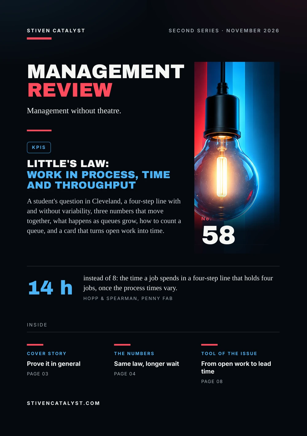
Stiven CatalystSecond series · November 2026
ManagementReview
Management without theatre.
KPIs
Little's law:work in process, time and throughput
A student's question in Cleveland, a four-step line with and without variability, three numbers that move together, what happens as queues grow, how to count a queue, and a card that turns open work into time.

No.58
14 h
instead of 8: the time a job spends in a four-step line that holds four jobs, once the process times vary.Hopp & Spearman, Penny Fab
stivencatalyst.com
No. 58 · KPIs
In this issue
Most reports show how much a team finished. Few show how much is still waiting, and fewer still connect the two with how long a customer waits. Little's law does: three averages, one equation, and no assumptions about how the work is done.
- 03Cover storyProve it in general
- 04The numbersSame law, longer wait
- 05The modelThree numbers, one equation
- 06What the research saysLess waiting, at a price
- 07How it is measuredCount the queue, find the time
- 08Tool of the issueFrom open work to lead time
- 09SourcesSources and method
How to read this issue
Figure
Every figure has its source and year at the foot of its page.
Our reading
Where the editors interpret rather than the research, it says so.
Practice
The steps and the card are proposals to try, not research results.
Cover story
Prove itin general
Around 1960 John Little taught queuing at the Case Institute of Technology in Cleveland. He told his class that one formula kept turning up in model after model and seemed very general. After class a student, Sid Hess, asked how hard it would be to prove it in general. Little's answer:
“I guess it shouldn't be too hard.”
01
L
the average number of items in the system, waiting or being served
02
λ
the average rate at which items arrive, per hour or per day
03
W
the average time an item spends in the system
“Famous last words,” he wrote fifty years later. The proof, worked out over summers on Nantucket, appeared in Operations Research in 1961: L = λW, whatever the pattern of arrivals, the service times or the order of service. Little's own explanation is simple: a person standing in a queue can be counted, and at the same time is collecting minutes of waiting.
Our reading
The law does not say how to shorten a queue. It says that the queue, the pace and the wait cannot be managed one at a time.
Sources: John D. C. Little, Operations Research 59(3), 2011; John D. C. Little, Operations Research 9(3), 1961
The story and the quotes come from Little's own account for the law's 50th anniversary (2011). The 1961 proof assumes stationary processes; in 2011 Little also proves the law for any finite period.
The numbers
Same law,longer wait
Wallace Hopp and Mark Spearman teach the law with the Penny Fab: four identical steps in a row, two hours each per penny. A job needs eight hours of work; the line can finish one every two hours. New jobs enter only to keep a set number inside.
Hours a job spends in the Penny Fab, by jobs in the line
Without variability, four jobs fill the line: one leaves every two hours, each after eight; more jobs only add waiting. With variable process times, four jobs bring out 0.286 an hour instead of 0.5, each after 14 hours. In every row, output per hour times hours inside gives back the number of jobs.
Our reading
Variability does not break the law. It raises the price: the same output needs more work in process, and every extra job is paid for in waiting.
Sources: Joan Tafoya & Tim Skowronski, Intel, IIE Conference, 2008; Wallace J. Hopp & Mark L. Spearman, Irwin/McGraw-Hill, 2000 (via Little (2011), section 4.2; Tafoya & Skowronski (2008))
A teaching example, not measured data: the Penny Fab tables shown by two Intel engineers in 2008, after Hopp and Spearman. Eight hours × 0.5 jobs an hour = the four jobs that fill the line.
The model
Three numbers,one equation
In operations, Hopp and Spearman put output first: throughput equals work in process divided by cycle time, the time a job spends between release and the end of its route. Little explains why: for an operating manager, output is usually the reason the operation exists, and it is often set from outside, by orders or a forecast.
01
Know two, find the third
The most common use: one number is hard to measure, the other two are not.
02
They move together
More output, shorter waits and less stock cannot be chosen one at a time.
03
Output fixed
Then the only way to cut work in process is to cut the time each item waits.
Each of the three numbers is a measure of performance on its own, Little writes, and managers should consider collecting and displaying all three for whatever stream of items they manage. If something is amiss, it will most likely show in one of them.
Our reading
A board that shows only what was finished hides two of the three numbers. Count what is open, and the waiting time follows from the arithmetic.
Sources: Wallace J. Hopp & Mark L. Spearman, Irwin/McGraw-Hill, 2000 (via Little (2011), section 4.2; Tafoya & Skowronski (2008)); John D. C. Little, Operations Research 59(3), 2011
Hopp and Spearman's terms as quoted by Little (2011); the three uses and the call to managers are Little's. The reading is the editors'.
What the research says
Less waiting,at a price
The law is exact, but it does not say how much work in process is right. Three reports show what practice adds to it.
Kanban teams, 2018
Dag Sjøberg studied more than 8,000 work items of five teams in one software company over four years. Less work in process went with shorter lead times, as the literature claims; more work in process also went with higher productivity. No single best limit emerged.
Emergency departments
Arrivals divided by what one doctor treats give the minimum staff: 10 patients an hour at 2.5 per doctor means 4 doctors. Because queues grow slowly at first and then fast as arrivals near capacity, the rule of thumb reported by Little adds 10–20%.
A server under load, 2010
In a load test, the queue of requests grew roughly in step with the load, then climbed steeply; above about 18 requests a second, more were essentially dropped. Little reads it as the large queue itself slowing the service.
Our reading
Full load looks efficient on a capacity chart. In the queue, it is where waiting stops growing in a straight line.
Sources: Dag I. K. Sjøberg, Proceedings of the 12th ACM/IEEE International Symposium on Empirical Software Engineering and Measurement (ESEM), 2018 (via Abstract at Semantic Scholar); John D. C. Little, Operations Research 59(3), 2011
Sjøberg's study covers one company and shows correlations; productivity was hard to measure. The two other cases are reported by Little (2011) from conversations with the people involved, not as independent studies.
More in the essayHigh-volume days: the standard under pressure
How it is measured
Count the queue,find the time
Practitioners always measure over a finite period, Little points out, and over any such period the law holds exactly. A team can measure two numbers and compute the third, or measure all three and check its data.
Draw the boundary
Where an item enters, where it leaves, and what counts as one item.
Count what is inside
At fixed times, every morning for example; average over the period.
Count what leaves
Per day or per hour, over the same period and in the same units.
Divide and compare
Inside ÷ leaving = average time inside. Set it against the times you have recorded.
Hypothetical example, a returns desk over four weeks
- Open each morning
- 60 cases on average
- Closed per day
- 20 cases on average
- Time inside
- 60 ÷ 20 = 3 working days
If the system's own timestamps say 1.5 days, a count is wrong, perhaps the cases on hold. The numbers are invented.
Source: John D. C. Little, Operations Research 59(3), 2011
The finite-period proof comes from Little (2011), as does Bill Lovejoy's remark, from a hospital study, that the law is a reality check on data that do not add up. The steps and the example are the editors'.
Tool of the issue
From open workt o lead time
One queue, one period. Count what is inside and what leaves, divide, and decide how much open work the team allows before it starts anything new.
01Queue and boundarywhere an item enters, where it leaves, which unit
02Periodfrom and to; the same dates for every count
03Work in processaverage count of open items; when and how counted
04Throughputitems finished per day over the period
05Lead time = work in process ÷ throughputin days; against recorded times and what customers are promised
06Limit and checkmost open items allowed; who holds new starts; when we count again
Sources: John D. C. Little, Operations Research 59(3), 2011; Mark L. Spearman, David L. Woodruff & Wallace J. Hopp, International Journal of Production Research 28(5), 1990 (via Abstract reprinted by the Project Production Institute, 2018); Joan Tafoya & Tim Skowronski, Intel, IIE Conference, 2008
A practice proposed by the editors, after Little (2011), the Penny Fab and CONWIP, Spearman, Woodruff and Hopp's pull system that keeps the work in process of a whole line constant.
Open the tool: Delay Analyzerstivencatalyst.com/tools/delay-analyzer/
Sources and method
Every figurehas a source.
The figures in this issue come from the sources below. The year shows how recent each one is.
- A Proof for the Queuing Formula: L = λWJohn D. C. Little, Operations Research 9(3), 1961https://doi.org/10.1287/opre.9.3.383
- Little's Law as Viewed on Its 50th AnniversaryJohn D. C. Little, Operations Research 59(3), 2011https://doi.org/10.1287/opre.1110.0940
- Factory Physics: Foundations of Manufacturing Management, 2nd editionWallace J. Hopp & Mark L. Spearman, Irwin/McGraw-Hill, 2000 · via Little (2011), section 4.2; Tafoya & Skowronski (2008)
- Factory Physics: A Fast Cycle Time Story (conference slides)Joan Tafoya & Tim Skowronski, Intel, IIE Conference, 2008https://beta.factoryphysics.com/wp-content/uploads/2023/02/factory_physics_application_at_intel.pdf
- An empirical study of WIP in kanban teamsDag I. K. Sjøberg, Proceedings of the 12th ACM/IEEE International Symposium on Empirical Software Engineering and Measurement (ESEM), 2018 · via Abstract at Semantic Scholarhttps://doi.org/10.1145/3239235.3239238
- CONWIP: a pull alternative to kanbanMark L. Spearman, David L. Woodruff & Wallace J. Hopp, International Journal of Production Research 28(5), 1990 · via Abstract reprinted by the Project Production Institute, 2018https://doi.org/10.1080/00207549008942761
Editorial method
Each figure was checked for its year, its publisher and what exactly it measures. Where the publisher's page could not be opened, the figure was checked against independent summaries and is marked “via”. The editors' interpretation is marked “Our reading”. Figures that could not be confirmed are not in the issue.
ManagementReview
Management without theatre.
Every issue, one management question, checked against the best research.
All issues
stivencatalyst.com/magazine/management-review.html
Management Review · No. 58 · November 2026 · Stiven Catalyst
Click or swipe a page to turn it. The arrow keys work too.
Management Review · No. 58
The figures of the issue
The charts of the printed pages, with their sources.
Source: Joan Tafoya & Tim Skowronski, Intel, IIE Conference, 2008
The whole text Read the issue as text For reading on a small screen, searching or a screen reader. The same words, without the page design.
In this issue
Most reports show how much a team finished. Few show how much is still waiting, and fewer still connect the two with how long a customer waits. Little's law does: three averages, one equation, and no assumptions about how the work is done.
In 1961 John Little proved a formula that teachers of queuing had met again and again: the average number of items in a system equals the rate at which they arrive times the average time each one stays. In Hopp and Spearman's four-step Penny Fab the law holds with and without variability, but the same work in process buys less output. In five Kanban teams, less work in process went with shorter lead times, and also with lower productivity. The card at the end turns a count of open work into a lead time.
Stiven Janaqi, Editor
Cover story
Prove it in general
Around 1960 John Little taught queuing at the Case Institute of Technology in Cleveland. He told his class that one formula kept turning up in model after model and seemed very general. After class a student, Sid Hess, asked how hard it would be to prove it in general. Little's answer:
I guess it shouldn't be too hard.
- L. the average number of items in the system, waiting or being served
- λ. the average rate at which items arrive, per hour or per day
- W. the average time an item spends in the system
“Famous last words,” he wrote fifty years later. The proof, worked out over summers on Nantucket, appeared in Operations Research in 1961: L = λW, whatever the pattern of arrivals, the service times or the order of service. Little's own explanation is simple: a person standing in a queue can be counted, and at the same time is collecting minutes of waiting.
Our reading
The law does not say how to shorten a queue. It says that the queue, the pace and the wait cannot be managed one at a time.
The story and the quotes come from Little's own account for the law's 50th anniversary (2011). The 1961 proof assumes stationary processes; in 2011 Little also proves the law for any finite period.
Sources: John D. C. Little, Operations Research 59(3), 2011; John D. C. Little, Operations Research 9(3), 1961
The numbers
Same law, longer wait
Wallace Hopp and Mark Spearman teach the law with the Penny Fab: four identical steps in a row, two hours each per penny. A job needs eight hours of work; the line can finish one every two hours. New jobs enter only to keep a set number inside.
Hours a job spends in the Penny Fab, by jobs in the line: 2 jobs: No variability 8, With variability 10; 4 jobs: No variability 8, With variability 14; 6 jobs: No variability 12, With variability 18.
Without variability, four jobs fill the line: one leaves every two hours, each after eight; more jobs only add waiting. With variable process times, four jobs bring out 0.286 an hour instead of 0.5, each after 14 hours. In every row, output per hour times hours inside gives back the number of jobs.
Our reading
Variability does not break the law. It raises the price: the same output needs more work in process, and every extra job is paid for in waiting.
A teaching example, not measured data: the Penny Fab tables shown by two Intel engineers in 2008, after Hopp and Spearman. Eight hours × 0.5 jobs an hour = the four jobs that fill the line.
Sources: Joan Tafoya & Tim Skowronski, Intel, IIE Conference, 2008; Wallace J. Hopp & Mark L. Spearman, Irwin/McGraw-Hill, 2000 (via Little (2011), section 4.2; Tafoya & Skowronski (2008))
The model
Three numbers, one equation
In operations, Hopp and Spearman put output first: throughput equals work in process divided by cycle time, the time a job spends between release and the end of its route. Little explains why: for an operating manager, output is usually the reason the operation exists, and it is often set from outside, by orders or a forecast.
- Know two, find the third. The most common use: one number is hard to measure, the other two are not.
- Th
e y movet oge ther. More output, shorter waits and less stock cannot be chosen one at a time. - Output fixed. Then the only way to cut work in process is to cut the time each item waits.
Each of the three numbers is a measure of performance on its own, Little writes, and managers should consider collecting and displaying all three for whatever stream of items they manage. If something is amiss, it will most likely show in one of them.
Our reading
A board that shows only what was finished hides two of the three numbers. Count what is open, and the waiting time follows from the arithmetic.
Hopp and Spearman's terms as quoted by Little (2011); the three uses and the call to managers are Little's. The reading is the editors'.
Sources: Wallace J. Hopp & Mark L. Spearman, Irwin/McGraw-Hill, 2000 (via Little (2011), section 4.2; Tafoya & Skowronski (2008)); John D. C. Little, Operations Research 59(3), 2011
What the research says
Less waiting, at a price
The law is exact, but it does not say how much work in process is right. Three reports show what practice adds to it.
- Kanban teams, 2018. Dag Sjøberg studied more than 8,000 work items of five teams in one software company over four years. Less work in process went with shorter lead times, as the literature claims; more work in process also went with higher productivity. No single best limit emerged.
- Emergency depa
r tments. Arrivals divided by what one doctor treats give the minimum staff: 10 patients an hour at 2.5 per doctor means 4 doctors. Because queues grow slowly at first and then fast as arrivals near capacity, the rule of thumb reported by Little adds 10–20%. - A server under load, 2010. In a load test, the queue of requests grew roughly in step with the load, then climbed steeply; above about 18 requests a second, more were essentially dropped. Little reads it as the large queue itself slowing the service.
Our reading
Full load looks efficient on a capacity chart. In the queue, it is where waiting stops growing in a straight line.
Sjøberg's study covers one company and shows correlations; productivity was hard to measure. The two other cases are reported by Little (2011) from conversations with the people involved, not as independent studies.
Sources: Dag I. K. Sjøberg, Proceedings of the 12th ACM/IEEE International Symposium on Empirical Software Engineering and Measurement (ESEM), 2018 (via Abstract at Semantic Scholar); John D. C. Little, Operations Research 59(3), 2011
More in the essay: High-volume days: the standard under pressure
How it is measured
Count the queue, find the time
Practitioners always measure over a finite period, Little points out, and over any such period the law holds exactly. A team can measure two numbers and compute the third, or measure all three and check its data.
- Draw the boundary. Where an item enters, where it leaves, and what counts as one item.
- Count what is inside. At fixed times, every morning for example; average over the period.
- Count what leaves. Per day or per hour, over the same period and in the same units.
- Divide and compare. Inside ÷ leaving = average time inside. Set it against the times you have recorded.
Hypothe tical example, a re turns desk over four weeks
- Open each morning: 60 cases on average
- Closed per day: 20 cases on average
- Time inside: 60 ÷ 20 = 3 working days
If the system's own timestamps say 1.5 days, a count is wrong, perhaps the cases on hold. The numbers are invented.
The finite-period proof comes from Little (2011), as does Bill Lovejoy's remark, from a hospital study, that the law is a reality check on data that do not add up. The steps and the example are the editors'.
Source: John D. C. Little, Operations Research 59(3), 2011
Tool of the issue
From open work t o lead time
One queue, one period. Count what is inside and what leaves, divide, and decide how much open work the team allows before it starts anything new.
- Queue and boundary where an item enters, where it leaves, which unit
- Period from and to; the same dates for every count
- Work in process average count of open items; when and how counted
- Throughput items finished per day over the period
- Lead time = work in process ÷ throughput in days; against recorded times and what customers are promised
- Limit and check most open items allowed; who holds new starts; when we count again
A practice proposed by the editors, after Little (2011), the Penny Fab and CONWIP, Spearman, Woodruff and Hopp's pull system that keeps the work in process of a whole line constant.
Sources: John D. C. Little, Operations Research 59(3), 2011; Mark L. Spearman, David L. Woodruff & Wallace J. Hopp, International Journal of Production Research 28(5), 1990 (via Abstract reprinted by the Project Production Institute, 2018); Joan Tafoya & Tim Skowronski, Intel, IIE Conference, 2008
Open the tool: Delay Analyzer
Sources and method
Every figure has a source.
The figures in this issue come from the sources below. The year shows how recent each one is.
- John D. C. Little, Operations Research 9(3), “A Proof for the Queuing Formula: L = λW”, 1961. https://doi.org/10.1287/opre.9.3.383
- John D. C. Little, Operations Research 59(3), “Little's Law as Viewed on Its 50th Anniversary”, 2011. https://doi.org/10.1287/opre.1110.0940
- Wallace J. Hopp & Mark L. Spearman, Irwin/McGraw-Hill, “Factory Physics: Foundations of Manufacturing Management, 2nd edition”, 2000 (via Little (2011), section 4.2; Tafoya & Skowronski (2008)).
- Joan Tafoya & Tim Skowronski, Intel, IIE Conference, “Factory Physics: A Fast Cycle Time Story (conference slides)”, 2008. https://beta.factoryphysics.com/wp-content/uploads/2023/02/factory_physics_application_at_intel.pdf
- Dag I. K. Sjøberg, Proceedings of the 12th ACM/IEEE International Symposium on Empirical Software Engineering and Measurement (ESEM), “An empirical study of WIP in kanban teams”, 2018 (via Abstract at Semantic Scholar). https://doi.org/10.1145/3239235.3239238
- Mark L. Spearman, David L. Woodruff & Wallace J. Hopp, International Journal of Production Research 28(5), “CONWIP: a pull alternative to kanban”, 1990 (via Abstract reprinted by the Project Production Institute, 2018). https://doi.org/10.1080/00207549008942761
Edit orial me thod
Each figure was checked for its year, its publisher and what exactly it measures. Where the publisher's page could not be opened, the figure was checked against independent summaries and is marked “via”. The editors' interpretation is marked “Our reading”. Figures that could not be confirmed are not in the issue.
Management Review · Monthly edition